
The receptor noise limited (RNL) chromaticity colour space is convenient because the Euclidean distance between any two points in this space is equal to the Delta-S of the RNL model (in units of “just noticeable differences”, JNDs). This means that if any two colours have a Euclidean distance of less than ~1-3 JNDs it is unlikely the two colours will be distinguishable. Where we know only a limited amount about the colour vision system of a given receiver this space is particularly useful and has been found to describe behavioural data well in a number of species (e.g. bees, humans, birds, lizard, and fish).
Input Requirements
This tool requires a 32-bit cone-catch image where the slice labels are named correctly (matching the names in the Weber fractions file for the visual system, or you can specify your own), and the channels should ideally go from longest to shortest wavelength sensitivity (this is the default for the toolbox).
Running the Tool
We recommend using the QCPA framework to perform this function, however you can run it on its own. Select a cone catch image and run:
plugins > micaToolbox > QCPA > Cone Catch to RNL Chromaticity
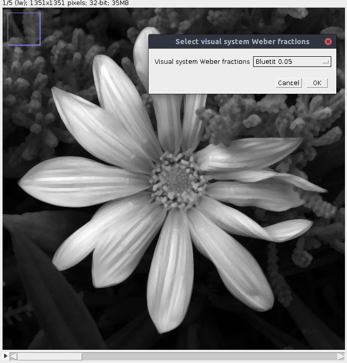
You will be asked to specify the Weber fractions for each channel. These are typically based on relative cone abundance if behavioural data are not available. You can either select the correct species (in which case the receptor names in the image and specification file must match, you will be notified if they do not), or specify you own. If the cone-catch image stack has a final luminance channel (as is required for the QCPA framework), this will be ignored appropriately.
Output
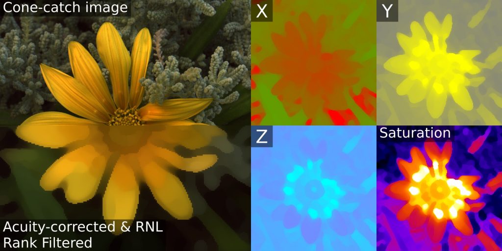
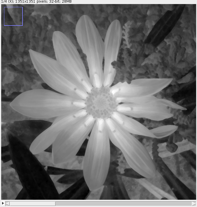
The output will vary depending on the number of receptor channels. Dichromatic cone-catch images will create a single “X” channel (showing opponency between LW and SW). Trichromatic cone-catch images will create a stack with an X and a Y channel (“X” is opponency between LW and MW (red-green), “Y” is opponency between the combination of LW and MW to SW (yellow-blue)). Tetrachromatic images are the same as trichromatic, but with a third “Z” channel, which is opponency between the combination of LW, MW and SW to UV.
The final slice shows saturation. This is the distance from each pixel’s XYZ coordinates to the achromatic point.
The output is simply a 32-bit greyscale stack suitable for measuring pixel values. Note you can also use these image for colour pattern analysis, such as measuring GabRat edge disruption. You may want to adjust the preview brightness/contrast of the stack.
To create a false-colour image like the ones at the top of this page follow these steps:
- Select the channel you wish to use from the output stack (e.g. X).
- Run Image > Duplicate and select only the current channel (do not tick the “Duplicate Stack” tickbox).
- Copy the current image (CTRL+C).
- Run Image > Stack > Add Slice.
- Paste: (CTRL+V).
- Run Process > Math > Multiply, and select “-1”. And select “No” when asked whether to process the entire stack.
- Run Image > Color > Make Composite, and select “Composite”.
- The default settings will now show a red-green opponent image. For a trichromat the RNL X channel is represented by red-green, and the RNL Y channel is blue-yellow. You can select whichever colours you want by selecting the first or second slice in the image stack and selecting a “lookup table”. e.g. Image > Lookup Tables > Yellow to select yellow. For a dichromat the X channel should be blue-yellow. For a trichromat X = red-green, Y = blue-yellow. Tetrachromats are the same as dishcromats, but the Z channel could e.g. be cyan-magenta.
- Importantly, the min and max viewing range must be set, and must be equal in positive and negative values (e.g. -10 and +10, or -30 and +30). If you do not do this the achromatic point will not be in the middle. Go Plugins > Measure > Set Min And Max, and choose values which give a suitable colour range. It’s important that whatever range you use is standardised and equal across images if you’re using these images to show differences between samples.
- The “Saturation” channel can simply be shown on its own in greyscale, or you can choose some other lookup table to show it. e.g. the example at the top of this page is using the “Fire” lookup table.
- With a lookup table applied and min & max values set you can simply save the current image as a JPG.