
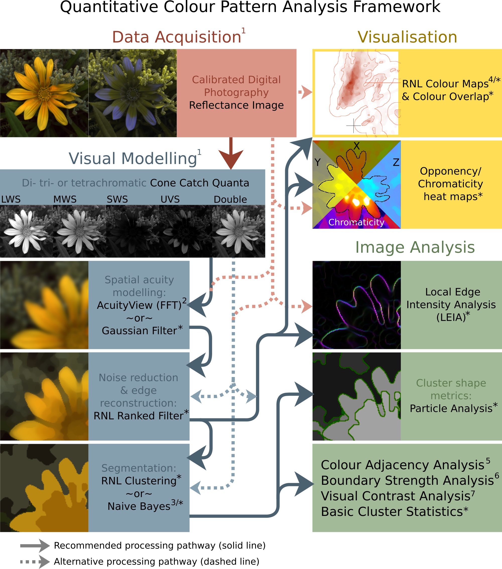
The Quantitative Colour and Pattern Analysis (QCPA) framework is an image processing workflow which takes an “animal vision” cone-catch image, applies spatial acuity and viewing distance correction, and then performs a series of sophisticated colour and pattern analysis procedures. Historically colour and pattern have been analysed separately, however this framework can perform analyses based on di- tri- and tetra-chromatic visual systems.
The framework uses the Vorobyev and Osorio (1998) Receptor Noise Limited (RNL) model throughout, which has been behaviourally validated in a range of species.
Many of the analysis procedures used by the QCPA framework require the image to be reduced to a small number of discrete colour patches, so the process can utilise novel image segmentation algorithms based on colour discrimination thresholds.
While there is a clear recommended processing pathway (see figure below) the framework is highly flexible, and can include or exclude various steps, and in many cases there are different options for achieving each step.
Video Guides
Input Requirements
The QCPA framework requires a 32-bits/channel cone-catch image. For acuity control you will need to know the receiver’s spatial acuity (see list), and also need a scale bar in the image (unless you know the image’s angular width). For RNL modelling (RNL Ranked filter, RNL clustering, and many of the analyses) you will need to know the Weber fractions for each receptor class, or failing that the approximate cone ratios (a range of species are included in the toolbox). For naive Bayes clustering you will either need to have a results table containing the mean and standard deviation of pixel values in each channel, for each patch, or two or more ROIs specified which will be measured and used for the naive Bayes clustering. Additionally, you can have a region of interest (ROI) specified, where – for example – you can analyse a section of the image completely independently of its background.
Note that the framework has various options to switch on or off different processing steps. So, for example, you could save the RNL Rank filtered image stack, and re-run the framework on this image stack (deselecting the processing steps up to and including RNL ranked filtering).
To create a cone-catch image you must generate or load a calibrated mspec image (linear normalised reflectance stack) and convert to cone catch using a model. The first slices in the stack must be the chromatic channels, with a final luminance slice in the stack. Here are examples of input image stacks for tetra-, tri- and di-chromatic modelling:
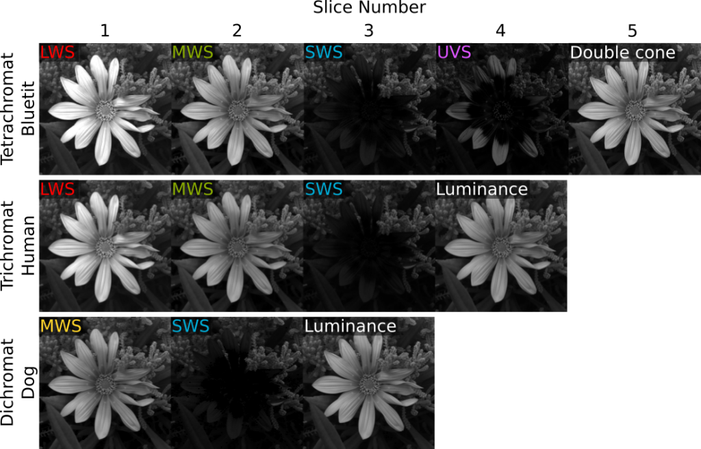
If the cone-catch model doesn’t create a final luminance channel automatically (e.g. the “double” cones in birds), you will need to add your own. This will vary between visual system. There is a tool provided for adding a luminance channel.
plugins > micaToolbox > Image Transform > Create Luminance Channel
This tool adds a final luminance channel at the end of the cone-catch image stack, based on an equal average of all the selected channels.
Any pixel with zero values or negative values in any channel is ignored in RNL Ranked filtering and clustering (the RNL model can’t deal with them, but this is also a method for screening out sections of the image which you do not want to include in clustering).
Running the QCPA Framework
Ensure the correct cone-catch image is selected and run:
plugins > micaToolbox > QCPA > Run QCPA Framework
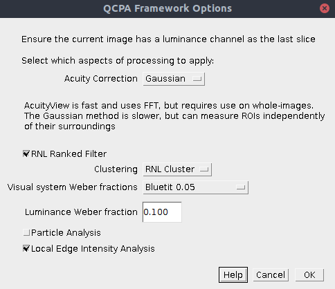
The first dialog box lets you select which components of the framework you wish to run. Subsequent dialog boxes will ask for component-specific settings (see the page for each for relevant information).
| Acuity Correction | AcuityView: Use the AcuityView method for controlling for spatial acuity. This uses FFT and a convolution in the frequency domain. As such, it can only be used on whole (rectangular) images. Any ROI will be smoothed with its surroundings. Gaussian: Use the custom-written Gaussian Acuity Control method. This uses a non-separable Gaussian convolution which is able to apply the appropriate level of smoothing on irregularly shaped ROIs completely independently of their surrounding pixels. |
| RNL Ranked Filter | Choose whether to apply the RNL Ranked filter. |
| Clustering | RNL Cluster: Use RNL clustering on the image. This breaks down the image into a discrete number of segments/clusters/patches based on visual models of colour and luminance discrimination. This the default option when you don’t know exactly how many patches there should be in your image. Naive Bayes Cluster: This uses naive Bayes clustering to segment the image. Use this option if you know exactly how many patches there should be in your image. You should either have a results table listing the mean and standard deviation of each patch and each channel, or have a number of ROIs in the ROI manager which can be used to create these values automatically. |
| Visual system Weber fractions | You can specify the Weber fractions of each channel for the given visual system. In the absence of behavioural data on each of these values, the receptor class with the most abundant cones is generally given the base Weber fraction (common values used are 0.05 or 0.1), and the less abundant receptor classes are given higher values based on cone abundance ratios. See Vorobyev & Osorio (1998) for details. A number of visual systems have been included by default, or you can select “Custom” to specify your own. If you really have no idea which numbers to use, then set every channel to 0.1 (not recommended) and make sure you declare the numbers used in any publication. |
| Luminance Weber Fraction | Specify the luminance Weber fraction. This will often be around 0.1 or 0.2, but varies with species and requires behavioural validation. If in doubt, select 0.1. |
| Particle Analysis | This will run the particle analysis following clustering, providing data on the shape and abundance of patches of each cluster. Additionally it outputs each cluster as a new ROI so that each can be measured independently if desired (e.g. select the RNL Ranked filtered image, and use the ROIs to measure different image regions based on automated clustering). |
| Local Edge Intensity Analysis | This will run the local edge intensity analysis, providing data similar to the boundary strength analysis, but on the un-clustered image. |
Output
The output will vary depending on the processing steps chosen, however if the entire framework is used the output will be:
- Spatial acuity-controlled cone-catch stack (this looks like a blurred image, which will have been scaled to the desired number of pixels-per-minimum-resolvable-angle). Note the ROIs are scaled to match this image, and all subsequent image. The original ROIs (saved with the mspec image) are unaffected.
- RNL Rank filtered cone-catch stack, where edges have been reconstructed following spatial acuity modelling. Measuring this image is recommended for creating colour maps. You can also make a colour presentation image of this image to show the results of spatial acuity modelling and edge reconstruction.
- Cluster cone-catch average stack (with the suffix “_Clustered”). This stack shows the average cluster value for the selected range of recorded passes. Use this image for creating a colour “presentation image” of the clustered image.
- Cluster ID image (with the suffix “_Cluster_IDs”). This image shows which cluster each pixel belongs to. The numbers correspond to the clusterID numbers in the “Cluster Results” window.
- Cluster Results table. This outputs the summary statistics for each cluster (e.g. average cone-catch value, RNL XYZ coordinates etc…) Optionally also shows the adjacency matrix (the number pixels where each cluster is found adjacent to every other cluster, used for various analyses).
- ROI Cluster Results table. As above, however this breaks down the cluster results by ROI, showing only the clusters which are present in each ROI.
- Summary Results table. This output contains the QCPA results from a large number of analyses which require a clustered image (e.g. boundary colour strength analysis, adjacency analysis and visual contrast analysis). Note that this analysis is repeated for each ROI in the image.
- Cluster Particle Analysis Summary Results table. Details information on the average shape/size descriptors of particles in each cluster.
- Individual Particle Results table. Shows shape/size descriptors for each individual particle (each cluster will often be composed of a number of particles)
- Local Edge Intensity Analysis images. Two images are produced for the chromatic LEIA (suffix “_Col_LEIA”) and luminance LEIA (suffix “_Lum_LEIA”). The false-colours show the angle of each edge, and the brightness shows the intensity of the edge. each image is a stack where each slice shows the results at different measured angles (vertical, horizontal and two diagonals).
- Local Edge Intensity Analysis results table. Shows the LEIA metrics.
- Log. The log shows exactly which steps were performed, and the user-controlled settings for each. Saving the log may be useful for remembering exactly which settings were used for a given analysis, and gives all the information required to reproduce your image analysis process which you should specify in any publication.
Summary Table Output Parameters
There are a large number of different numbers produced by the QCPA analysis, each describing different image properties. The table below gives a very brief description of each of these variables. For specific details and equations, please see the Appendix released with the QCPA publication. The default output shows the horizontal and vertical matrix analyses combined, however most of the variables can also be split into separate values by ticking the relevant box during processing (see above). If you are interested in comparing horizontal and vertical values separately (e.g. because pattern orientation is interesting in your study system), then make sure all of your images are rotated to a uniform orientation before analysis.
| Abbreviation | Variable Name |
| CAA:Sc | Simpson colour diversity – Sc (eq. 1). This describes how evenly different colours in an image are represented, in terms of area coverage. The higher the number of different colours (number of discrete colour clusters), the higher the potential maximum value of Sc (up to the number of different colours). |
| CAA:Jc | Relative Simpson colour diversity – Jc (eq. 2). As above, but controlling for the number of different colours, so describes how evenly the colours are represented (in terms of area) independent of the number of colours. |
| CAA:St | Simpson transition diversity – St (eq. 3). This describes the regularity of transitions between different colours in an image. St is equal to the number of different colours when all transitions are equally frequent. |
| CAA:Jt | Relative Simpson transition diversity – Jt (eq. 4). As above, but controlling for the number of different colours, so describes how evenly the colours transition independent of the number of colours. |
| CAA:Hc | Shannon colour diversity – Hc (eq. 5). Also referred to as “entropy”, this is similar to Sc above, but uses a different diversity index. |
| CAA:Qc | Relative Shannon colour diversity – Qc (eq. 6). As above, but controlling for the number of different colours, so describes how evenly the colours are represented (in terms of area) independent of the number of colours, with a maximum value of 1. |
| CAA:Ht | Shannon transition diversity – Ht (eq. 7). This describes the regularity of transitions between different colours in an image (using the Shannon rather than Simpson index). Ht is equal to the number of different colour clusters when all transitions are equally frequent. |
| CAA:Qt | Relative Shannon transition diversity – Qt (eq.8). As above, but controlling for the number of different colours, so describes how evenly the colours transition independent of the number of colours, with a maximum value of 1. |
| CAA:Scpl | Simpson colour pattern complexity Scpl (eq. 9). This combines Jt and Jc (colour diversity and transition diversity respectively), such that colour patterns with uniform spacing and coverage (such as a chessboard) would have a maximum value of 1. |
| CAA:Qcpl | Shannon colour pattern complexity Qcpl (eq. 10). As above, using Shannon instead of Simpson indices. |
| CAA:C | Pattern Complexity – C (eq. 11). This describes the geometric complexity of colour patterns based on the number of same-colour and different-colour transitions. Patterns with more complex structures will have higher values. |
| CAA:PT | Average patch size – PT. The average patch size of each colour based on horizontal and vertical “run lengths” of each colour (note that the particle analysis tool may be more informative). |
| CAA:PT Hrz | Average horizontal patch size – PTHrz . The average “run length” (in pixels) of horizontal colour patches. |
| CAA:PT Vrt | Average vertical patch size – PTVrt . The average “run length” (in pixels) of vertical colour patches. |
| CAA:Asp | Aspect ratio – A. 0 implies horizontally elongated patterns, 0.5 indicates equal circular or random patterns, 1 indicates vertically elongated patterns. |
| VCA:ML | Weighted mean of pattern luminance contrast – ML (eq. 13) The mean luminance of the image (weighted by the area of each colour). |
| VCA:sL | Weighted standard deviation of pattern luminance contrast – sL (eq. 14). Standard deviation of the luminance of the image (weighted by the area of each colour). Higher values imply more variance in luminance values. |
| VCA:CVL | Weighted CoV of pattern luminance contrast – CVL (eq. 15) Coefficient of variation of luminance in the image (based on the above two values). Higher values imply more variance, while controlling for the mean value. |
| VCA:MDmax | Weighted mean of pattern Dmax contrast – MDmax (eq. 16) The mean Dmax contrast of the image (weighted by the area of each colour). Dmax is the most stimulated pairwise opponent channel (a colour channel which describes chromaticity, i.e. both hue and saturation) of each colour relative to grey (the achromatic point). Consider using the RNL saturation-based values instead for well characterised visual systems because it is a more perceptually uniform colour space. |
| VCA:sDmax | Weighted standard deviation of pattern Dmax contrast – sDmax (eq. 17). Standard deviation of the Dmax contrast of the image (weighted by the area of each colour). Higher values imply more variance in Dmax chromaticity values, and a more “colourful” image. |
| VCA:CVDmax | Weighted CoV of pattern Dmax contrast – CVDmax (eq. 18). Coefficient of variation of Dmax contrast in the image (based on the above two values). Higher values imply more variance, while controlling for the mean value. |
| VCA:MSsat | Weighted mean of pattern RNL saturation contrast – ΔSSat (eq. 19). The mean RNL saturation of the image (weighted by the area of each colour). RNL saturation is the distance (in receptor noise limited space, Vorobyev & Osorio 1998) of each colour from grey (the achromatic point). E.g. a fairly uniformly bright “red” image will have a high overall saturation, and a grey image will have a low value. Images with extremely varied colours (e.g. red, green and blue equally weighted) will also have a low mean, but high variance (see below). |
| VCA:sSsat | Weighted standard deviation of pattern RNL saturation contrast – sΔSSat (eq. 20). Standard deviation of the RNL saturation of the image (weighted by the area of each colour). Higher values imply more variance in RNL saturation values, and a more “colourful” image relative to grey. See also the VCA:MS value, which measures the internal differences between colours (i.e. colourful relative to each-other, instead of relative to grey). |
| VCA:CVSsat | Weighted CoV of pattern RNL saturation – CVSSat (eq. 21). Coefficient of variation of RNL saturation in the image (based on the above two values). Higher values imply more variance, while controlling for the mean value. |
| VCA:MSL | Weighted mean of RNL luminance pattern contrast – MSL (eq. 22). This is the average RNL luminance difference between all of the colours in the image, weighted by the area covered by each colour. Contrasts use the Siddiqi et al. 2004 method. Higher values imply larger luminance differences between colours in the image. |
| VCA:sSL | Weighted standard deviation of RNL luminance pattern contrast – sΔSL (eq. 23). The standard deviation of RNL luminance differences between all of the colours in the image, weighted by the area covered by each colour. Higher values imply larger variance in internal luminance differences, e.g. lots of similar and dissimilar luminance differences. |
| VCA:CVSL | Weighted CoV of RNL luminance pattern contrast – CVSL(eq. 24). Coefficient of variation of internal RNL luminance differences in the image (based on the above two values). Higher values imply more variance, while controlling for the mean value. |
| VCA:MS | Weighted mean of pattern RNL chromaticity contrast – MΔS (eq. 25). This is the average colour difference between all of the colours in the image, weighted by the area covered by each colour. Contrasts use the Vorobyev & Osorio 1998 Receptor Noise Limited method. Higher values imply larger internal colour differences between colours in the image. Therefore an image with lots of different colours will have a high value, irrespective of how far those colours are from the grey point. E.g. if the entire image is fairly uniformly bright “red” this value will be low, because all of the internal colours are similar. However, the saturation of the image (e.g. MSsat above) will be high. |
| VCA:sS | Weighted standard deviation of pattern RNL chromaticity contrast – sΔS (eq. 26). The standard deviation of RNL colour differences between all of the colours in the image, weighted by the area covered by each colour. Higher values imply larger variance in internal colour differences, e.g. lots of similar and dissimilar colours. |
| VCA:CVS | Weighted CoV of pattern RNL chromaticity contrast – CVΔS (eq. 27). Coefficient of variation of internal RNL colour differences in the image (based on the above two values). Higher values imply more variance, while controlling for the mean value. |
| BSA:BML | Weighted mean of luminance boundary strength – BML (eq. 28). The average luminance difference (based on Michelson contrasts) of boundaries between colours across the image, weighted by the relative frequency of transitions between each potential colour combination. Higher values imply higher luminance differences across colour boundaries. |
| BSA:BsL | Weighted standard deviation of luminance boundary strength – BsL (eq. 29). The standard deviation of luminance differences (based on Michelson contrasts) of boundaries between colours across the image, weighted by the relative frequency of transitions between each potential colour combination. Higher values imply higher variance in luminance differences across colour boundaries. |
| BSA:BCVL | Weighted CoV of luminance boundary strength – BCVL (eq. 30). Coefficient of variation of luminance differences of boundaries in the image (based on the above two values). Higher values imply more variance, while controlling for the mean value. |
| BSA:BMDmax | Weighted mean of Dmax boundary strength – BMDmax (eq. 31). The average Dmax chromaticity difference (based on Michelson contrast) of boundaries between colours across the image, weighted by the relative frequency of transitions between each potential colour combination. Higher values imply higher Dmax chromaticity differences across colour boundaries. Dmax is the most stimulated pairwise opponent channel (a colour channel which describes chromaticity, i.e. both hue and saturation) of each colour relative to grey (the achromatic point). Consider using the RNL saturation instead (below), which is closer to a perceptually uniform colour space. |
| BSA:BsDmax | Weighted standard deviation of Dmax boundary strength – BsDmax (eq. 32). The standard deviation of Dmax chromaticity differences of boundaries between colours across the image, weighted by the relative frequency of transitions between each potential colour combination. Higher values imply higher variance in Dmax differences across colour boundaries. |
| BSA:BCVDmax | Weighted CoV of Dmax boundary strength – BCVDmax (eq. 33). Coefficient of variation of Dmax chromaticity differences of boundaries in the image (based on the above two values). Higher values imply more variance, while controlling for the mean value. |
| BSA:BMSsat | Weighted mean of RNL saturation boundary strength – BMSSat (eq. 34). The average RNL saturation difference (i.e. the distance of each colour from the grey point, compared using Michelson contrast) of boundaries between colours across the image, weighted by the relative frequency of transitions between each potential colour combination. Higher values imply higher RNL saturation differences across colour boundaries. |
| BSA:BsSsat | Weighted standard deviation of RNL saturation boundary strength – BsSSat (eq. 35). The standard deviation of RNL saturation differences of boundaries between colours across the image, weighted by the relative frequency of transitions between each potential colour combination. Higher values imply higher variance in RNL saturation across colour boundaries. |
| BSA:BCVSsat | Weighted CoV of RNL saturation boundary strength – BCVSSat (eq. 36). Coefficient of variation of RNL saturation differences of boundaries in the image (based on the above two values). Higher values imply more variance, while controlling for the mean value. |
| BSA:BMSL | Weighted mean of RNL luminance boundary strength – BMSL (eq. 37). The average RNL luminance difference (using the Siddiqi et al. 2004 method) of boundaries between colours across the image, weighted by the relative frequency of transitions between each potential colour combination. Higher values imply higher luminance differences across colour boundaries. Consider using the “LEIA” method instead, which is similar but does not require a clustered image. |
| BSA:BsSL | Weighted standard deviation of RNL luminance boundary strength – BsSL (eq. 38). The standard deviation of RNL luminance differences of boundaries between colours across the image, weighted by the relative frequency of transitions between each potential colour combination. Higher values imply higher variance in luminance difference across colour boundaries. |
| BSA:BCVSL | Weighted CoV of RNL luminance boundary strength – BCVSL (eq. 39). Coefficient of variation of RNL luminance differences of boundaries in the image (based on the above two values). Higher values imply more variance, while controlling for the mean value. |
| BSA:BMS | Weighted mean of RNL chromaticity boundary strength – BMΔS (eq. 40). The average RNL colour difference (based on Vorobyev & Osorio 1998) of boundaries between colours across the image, weighted by the relative frequency of transitions between each potential colour combination. Higher values imply higher colour differences across colour boundaries. Consider using the “LEIA” method instead, which is similar but does not require a clustered image. |
| BSA:BsS | Weighted standard deviation of RNL chromaticity boundary strength – BsΔS (eq. 41). The standard deviation of RNL colour differences of boundaries between colours across the image, weighted by the relative frequency of transitions between each potential colour combination. Higher values imply higher variance in colour difference across colour boundaries. |
| BSA:BCVS | Weighted CoV of RNL chromaticity boundary strength – BCVΔS (eq. 42). Coefficient of variation of RNL colour differences of boundaries in the image (based on the above two values). Higher values imply more variance, while controlling for the mean value. |
Rotating Your Images
The pattern analyses (CAA/VCA/BSA) are very sensitive to the orientation of an image/ROI. Therefore, to ensure that measured pattern parameters are as comparable between images as possible, make sure you rotate your image into a uniform orientation prior to analysis.
The best way to do this is AFTER creating the .mspec but BEFORE applying a cone mapping model or any other edits. To rotate the image correctly choose the following settings:
Go to ‘image’ -> ‘Transform’ -> ‘Rotate…’ Select ‘Preview’ and ‘Zoom to fit’. Align the animal/ROI using the grid lines displayed. Make sure nothing gets clipped unless desired. If you have made any ROI selections prior to rotating the image you will have to redo them.
Avoiding Error Messages and other Malfunctions
File name length
Windows (And any other OS) has a maximum path length of 260 characters. This is quickly used up if you save your images with the full name QCPA has given it, especially when you operate in a directory that is multiple folders inside other folders. Make sure you avoid issues by trying to keep file names as short as possible.
Keeping things clean
MICA can have issues executing commands if you have old files open which are not necessary for your current project (e.g. another blurred image). Make sure you save and close any files that are not directly related to the current script you are trying to run.
Tipps to Increase Reproducibility
In addition to details outlined here, when modifying your images:
- Save the log file with your images to keep track of any changes
- Save your ROIs in the ROI manager by clicking ‘more’ -> ‘save’ and save your ROIs in a folder together with a given image. That way you will only select your ROIs once and the output will always be the same. You can load your ROIs by clicking ‘more’ -> ‘load’.
Citation & Reporting
If you use the QCPA framework you must cite our (forthcoming) paper. Note that you should also report the image analysis settings used in any publication. These are provided in the log window.
References:
Vorobyev, M., & Osorio, D. (1998). Receptor noise as a determinant of colour thresholds. Proceedings of the Royal Society of London. Series B: Biological Sciences, 265(1394), 351–358.
Siddiqi, A., Cronin, T. W., Loew, E. R., Vorobyev, M., & Summers, K. (2004). Interspecific and intraspecific views of color signals in the strawberry poison frog Dendrobates pumilio. Journal of Experimental Biology, 207(14), 2471–2485.