
We provide tools for performing a pattern analysis based on Fast Fourier bandpass filtering, often called a granularity analysis. This form of analysis is increasingly widely used to measure animal markings (Godfrey et al., 1987; Stoddard and Stevens, 2010), and is loosely based on our understanding of low-level neuro-physiological image processing in numerous vertebrates and invertebrates. Each image is filtered at multiple spatial frequency scales, and the “energy” at each scale is measured as the standard deviation of the filtered pixel values. The pattern energy of non-rectangular regions of interest are measured by extracting the selection so that all surrounding image information is removed (i.e. the selection area is measured against a black background). This image is duplicated and the selection area is filled with the mean measured pixel value (to remove all pattern information inside the selection area). Identical bandpass filtering is performed on both images and the difference between the images is calculated before measuring its energy for a shape-independent measure of pattern.
To perform pattern analysis using the batch measurement tool one must first select which channel to use for pattern analysis. Pattern processing in humans is thought to rely on the luminance channel (which is the combination of LW and MW sensitivities) and double cones in birds (Osorio and Vorobyev, 2005). If images are not being converted to cone catch quanta then the green channel is recommended (Spottiswoode and Stevens, 2010), or a combination of red and green (which is available as an automated option). Next, the desired measurement scales must be selected in pixels, along with the desired incrementation scale (e.g. linear increases of two pixels would provide measurements at 2, 4, 6, 8 pixels, and so on). A multiplier can be used instead, for example multiplying by two to yield measurements at 2, 4, 8 16 pixels and beyond. A size no larger than the scaled image dimensions should be used to cover the entire available range. The number of scale increments should be judged based on processing speed, although increasing the number of scales measured will yield progressively less additional information. We find that increasing the scale from 2 by a multiple of √2 up to the largest size available in the scaled images produces good results in many situations.
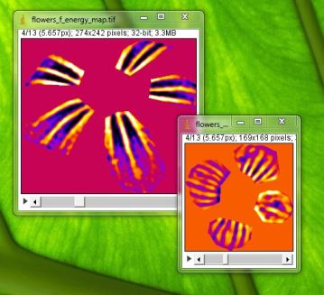
Summary statistics (Chiao et al., 2009; Stoddard and Stevens, 2010) of the pattern analysis are saved for each region of interest (or pooled regions). These include the maximum frequency (the spatial frequency with the highest energy; i.e. corresponding to the dominant marking size), the maximum energy (the energy at the maximum frequency), summed energy (the energy summed across all scales, or amplitude; a measure of pattern contrast), proportion energy (the maximum energy divided by the summed energy; a measure of pattern diversity, or how much one pattern size dominates), mean energy and energy standard deviation. In addition the energy spectra (the raw measurement values at each scale) can be output and used for pattern difference calculations (see below). Pattern maps can also be created – these are false colour images (Image 1) of the filtering at each scale – produced for subjectively visualising the process.
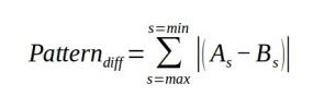
Animal markings and natural scenes often have pattern energy spectra with more than one peak frequency, meaning the pattern descriptive statistics (above) can arbitrarily jump between peaks with similar energy levels in different samples (Image 2). An alternative approach we recommend when directly comparing two samples, rather than deriving intrinsic measurements to each sample, is to calculate the absolute difference between two spectra (A and B) across the spatial scales measured s:
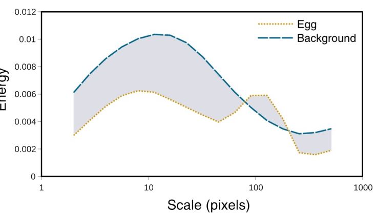
This is equivalent to the area between the two curves in Image 2. Any two patterns with very similar amounts of energy across the spatial scales measured will produce low pattern difference values irrespective of the shape of their pattern spectra. These differences will rise as the spectra differ at any frequency. As with colour, these differences can be calculated automatically between regions of interest, within or between images from the pattern energy spectra (above) using the “Pattern and Luminance Distribution Difference Calculator”. Luminance distribution differences are calculated similarly, summing the differences in the number of pixels in each luminance bin across the entire histogram. This method for comparing luminance is recommended when the regions or objects being measured do not have a normal distribution of luminance levels. For example, many animal patterns have discrete high and low luminance values (such as zebra stripes or egg maculation), in which case a mean value would not be appropriate. Comparing the luminance histograms overcomes these distribution problems.
References:
Chiao, C.-C., Chubb, C., Buresch, K., Siemann, L., and Hanlon, R.T. (2009). The scaling effects of substrate texture on camouflage patterning in cuttlefish. Vision Res. 49, 1647 – 1656.
Godfrey, D. Lythgoe, J.N., and Rumball, D.A. (1987). Zebra stripes and tiger stripes: the spatial frequency distribution of the pattern compared to that of the background is significant in display and crypsis. Biol. J. Linn. Soc. 32, 427-433
Stoddard, M.C., and Stevens, M. (2010). Pattern mimicry of host eggs by the common cuckoo, as seen through a bird’s eye. Proc. R. Soc. B Biol. Sci. 277, 1387-1393