
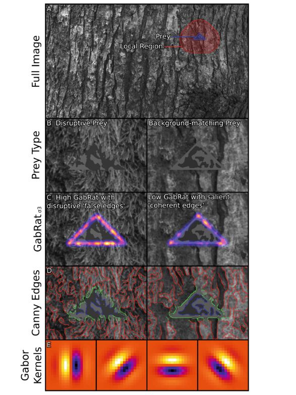
GabRat is a method developed for measuring the level of edge disruption around a given target. The method uses Gabor filtering, and measures the ratio (hence “Gabor -ratio” > GabRat) of the targets’ “true” outline edge intensity, compared to the intensity of any orthogonal “false edges” (which run at 90 degrees to the target’s outline). A higher ratio of false edges which run counter to the target’s outline create higher levels of edge disruption, and was found to be by far the best predictor of detection times in an experiment where humans were searching for camouflaged items (Troscianko et al. 2017).
Input Requirements
GabRat can be used on almost any image: calibrated mspec images, cone-catch images, CIELAB or RNL chromaticity (XYZ) images are recommended. The latter two are interesting because they allow you to measure chromatic edge disruption. There are two version of the tool. The first will go through each ROI in the ROI manager and provide GabRat measurements for each ROI in each image channel separately. The second version will only measure the currently selected ROI in the current image channel. If the processing throws up an error, it is likely because the edge of the target is too close to the edge of the image given the scale of the Gabor filter being used. Reduce the sigma value, or ensure any targets are not too close to the image boundaries.
The input image should ideally be scaled to match the viewer’s peak acuity contrast sensitivity (note this is different from an animal’s spatial acuity limit). To do this, find the acuity at which you expect the peak contrast sensitivity (e.g. see Souza et al. 2011 for a list of species peak contrast sensitivity values). Then scale the image using the QCPA framework, selecting only the first acuity correction step (either AcuityView or Gaussian acuity control). Ensure the output image is scaled to 5 pixels per minimum resolvable angle. This will automatically scale the image and all of its ROIs, creating a blurred, scaled image (do not apply RNL ranked filter or clustering). Now run the GabRat filter on the acuity controlled image with a sigma matching the px/MRA value (i.e. 5).
Run GabRat Measurement Tools
The recommended method for running GabRat measurements is with:
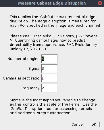
plugins > micaToolbox > Image Analysis > GabRat Disruption ROIs
You should have already specified any targets you wish to measure by creating ROIs for each of them. The tool will measure the GabRat of each target across all image slices.
However, in order to access some additional options (such as outputting the kernels, masks, and outline disruption measurements) you can also run:
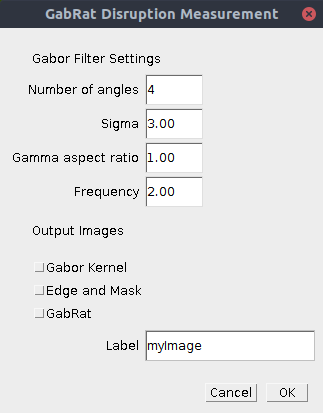
plugins > micaToolbox > Tools > Gabrat Disruption
This will only measure the current slice in an image stack, but will give you extra output for debugging, or visualising the GabRat filter (see table below).
| Number of Angles | Specify the number of angles for the Gabor filter. The default of 4 is generally sufficient and this will measure angles in the vertical (|), diagonal (/), horizontal (-) and other diagonal (\). |
| Sigma | Sigma is generally the only number you will want to change. This specifies the overall scale of the Gabor filters (larger sigma = larger filter/kernel). Ideally you would match the sigma size to the receiver’s peak contrast sensitivity function if this is known (note, this is different to the species visual acuity limit, see Souza et al. 2011). We recommend using an image which has been scaled to the receiver’s spatial acuity or one which has been scaled to a specific size (number of pixels per millimetre). To measure the disruption at the visual acuity limit selected, use a sigma value equal to the number of pixels per minimum resolvable angle chosen when scaling the image. A value of 5 pixels per MRA is recommended, in which case a sigma of 5 is also recommended. |
| Gamma Aspect Ratio | This changes the shape of the Gabor filter, use the “GabRat Disruption” tool (without the ROI) to output the kernel and play with the shape. The default value of 1 is recommended. |
| Frequency | This changes the frequency of the Gabor filter. A higher number will have more waves in the kernel. 2 is recommended, and fits with the receptive fields of edge detector neurophysiology. |
| Output Gabor kernel | This and the following options are only available in the standalone version of the tool (second tool shown above). If ticked it will output a stack of the Gabor kernel at different angles. |
| Edge and Mask | If ticked an additional stack showing the mask (an image showing where the target is and is not), and outline of the target ROI will be shown. |
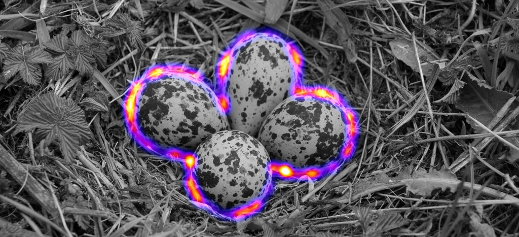
| GabRat | If ticked this will output a slice showing the GabRat value at each point around the edge of the target ROI. This can be used identify specific locations with low or high disruption, and to create a false-colour image of the GabRat intensity around the edge of the image (like the image at the top of this page). To create this presentation image, use a Gaussian blur on this output image equal to the sigma value used above. Then set the min and max appropriately and choose a suitable LUT (lookup table). Then overlay this image on the original (e.g. copy the GabRat image, then set the paste mode to “Add”, and paste over the original greyscale image). |
Output
If using the standard tool, the GabRat value will be measured for each slice in the image. If using the standalone tool (second tool above) you have the option for extra output images, useful for debugging, interpreting, and visualising the output.
Citation
If you use any GabRat measurements please cite:
Troscianko J., Skelhorn, J., & Stevens M. (2017). Quantifying camouflage: how to predict detectability from appearance. BMC Evolutionary Biology. 17:7. – link (open access) – Blog Post –
References
Souza, G. da S., Gomes, B. D., & Silveira, L. C. L. (2011). Comparative neurophysiology of spatial luminance contrast sensitivity. Psychology & Neuroscience, 4(1), 29–48. doi:10.3922/j.psns.2011.1.005