
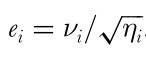
The noise in an individual photoreceptor cell (its firing rate despite lacking actual stimulation) in combination with the abundance of a given class of photoreceptors fundamentally determines an animal’s ability to discriminate colour and luminance contrast (Vorobyev & Osorio, 1998). The more photoreceptors of a given class a retina contains, the more likely it is that input from these receptors is being integrated to result in a higher sensitivity. Thus, it’s important to distinguish between the noise in a single photoreceptor and how that noise translates into channel-specific noise as a function of the relative receptor abundance:
This channel specific standard deviation of noise is often described as a Weber fraction (Norwich, 1987), although the original 1998 publication of the receptor limited (RNL) model does not use that term. The term Weber fraction is introduced in Vorobyev et al. 2001:
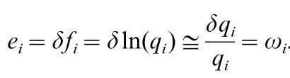
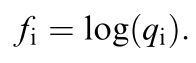
Where f(i) is the signal of receptor mechanism i, q(i) is the von-Kries adapted receptor quantum catch and δ is the standard deviation. From Vorobyev et al. (2001)
Vorobyev et al. (2001) state that the substitution of e(i) by ω(i) is only valid for colours which are close to the background colour as well as an unknown relation between receptor signals and quantum catches. Also, note the log transformation of the quantum catch q(i). Therefore, it’s only appropriate to equate the standard deviation of the noise in a channel to the Weber fraction in the log-transformed RNL model (Vorobyev et al. 2001). As Vorobyev et al. (1998) put it: “[using log-transformed quantum catches] gives the Fechner law”. QCPA exclusively uses the log-transformed RNL model which is why we refer to Weber fractions.
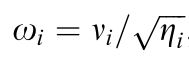
This terminology seems overwhelming but it is important to adhere to for the sake of reproducible research. However, the terminology has recently been further confused by other authors. For example, Renoult et al. (2017) where e(i) is called the ‘photoreceptor noise’ which according to them is to be calculated using the following equation:
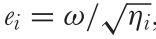
Where e(i) is the ‘Photoreceptor noise’, ω(i) is the ‘Weber fraction’ and η(i) is the ‘relative density of photoreceptor i‘. In other words: They propose using the ‘Weber fraction’ (which Vorobyev & Osorio (1998) called the receptor specific noise) for both the linear and log-linear RNL model while calling the channel specific standard deviation of noise (e(i)) ‘receptor noise’ despite using the same symbol as Vorobyev & Osorio (1998) while using what they call a ‘Weber fraction’ in the place of what should be the receptor specific noise to calculate what they call ‘neural noise’ which Vorobyev & Osorio called channel specific noise.
Confusing, right? Thus, to avoid confusion, we propose strictly adhering to the original definitions of Vorobyev & Osorio 1998, Vorobyev et al. 1998 and Vorobyev et al. 2001.
How to calculate channel-specific standard deviations of noise (or Weber fractions)
There is very little insight provided in the literature on how to actually arrive at correctly calculating e(i) or ω(i).
First, we need to obtain relative cone abundances for the retinal area of interest. These are usually expressed as ratios relative to the least abundant cone. e.g. 1:2:2 for sw:mw:lw meaning for each sw (shortwave sensitive) receptor there are two of each mw (mediumwave) and lw (longwave). These values (as opposed to receptor noise values which are extremely rare) can be found in the literature comparably easy.
Second, we need to reverse the normalisation of the cone ratios we got from our retinal map so that the most abundant class becomes 1. e.g. 1:2:2 becomes 0.5:1:1. This is equivalent to the assumption that the most abundant receptor type creates the least noisy channel and all the less abundant receptor types create noisier channels.
Third, we use the square root of these new cone ratios to divide our noise level in our single photoreceptor by (see first equation on top of page). e.g. in our example we assume a receptor noise of 0.05 which gives us 0.07:0.05:0.05 for sw:mw:lw. E.g. the sw channel is noisier because it’s less abundant. 0.05 is a fairly conservative receptor noise estimate often used in the literature if actual receptor noise is not known (which it rarely is).
In order for visual modelling to be reproducible this information needs to be provided. This is often not done in the literature and is a bad habit.
References:
Renoult, J.P., Kelber, A. & Schaefer, H.M. 2017. Colour spaces in ecology and evolutionary biology. Biol. Rev. 92: 292–315.
Norwich, K. H. (1987). On the theory of Weber fractions. Perception & Psychophysics, 42(3), 286–298.
Vorobyev, M., Osorio, D., Bennett, a. T.D., Marshall, N.J. & Cuthill, I.C. 1998. Tetrachromacy, oil droplets and bird plumage colours. J. Comp. Physiol. – A Sensory, Neural, Behav. Physiol. 183: 621–633.
Vorobyev, M., Brandt, R., Peitsch, D., Laughlin, S.B. & Menzel, R. 2001. Colour thresholds and receptor noise: Behaviour and physiology compared. Vision Res. 41: 639–653.
Vorobyev, M. & Osorio, D. 1998. Receptor noise as a determinant of colour thresholds. Proc. R. Soc. B Biol. Sci.265: 351–358.