
The RNL clustering technique was developed specifically for the QCPA workflow, parts of which require a colour image be segmented into different pattern elements or ‘clusters’. Unlike previous approaches this technique uses log receptor noise limited (RNL) modelling of Delta-S distances and perceptual thresholds (which can be behaviourally validated), for chromatic (colour) and achromatic (luminance) clustering.
Advantages:
- The algorithm uses animal vision modelling when deciding whether any two colour patches will be combined.
- The algorithm only needs to be told what perceptual thresholds are required for the given visual system, you do not need to know how many different pattern elements or clusters there are in the image (unlike naive Bayes or k-mean clustering, for example).
- The algorithm supports di- tri- and tetrachormatic visual systems.
- The influence of colour and luminance can be combined or separated in clustering.
- There is no random element to the clustering – the same input will always create the same output with constant settings – and the method is robust against image rotation.
- Increasing the size of the receptive field, while simultaneously decreasing the number of discrete clusters is computationally efficient, and matches plausible colour processing steps in the brain.
- Clustering can be performed on a sub-section of any image (with ROIs of any shape).
Input Image
We recommend this method should be used following acuity control (FFT-based AcuityView or Gaussian acuity control) and RNL ranked filtering. RNL clustering requires a cone-catch image stack. To create a cone-catch image you must generate or load a calibrated mspec image and convert to cone catch using a model. The first slices in the stack must be the chromatic channels, with a final luminance slice in the stack. Here are examples of input image stacks for tetra-, tri- and di-chromatic modelling:
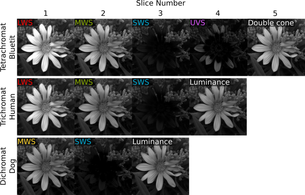
If the cone-catch model doesn’t create a final luminance channel automatically (e.g. the “double” cones in birds), you will need to add your own. This will vary between visual system. There is a tool provided for adding a luminance channel.
plugins > micaToolbox > Image Transform > Create Luminance Channel
This tool adds a final luminance channel at the end of the cone-catch image stack, based on an equal average of all the selected channels.
Any pixel with zero values or negative values in any channel is ignored in clustering (the RNL model can’t deal with them, but this is also a method for screening out sections of the image which you do not want to include in clustering).
Running RNL Clustering
With the appropriate image open in ImageJ, we recommend running the QCPA framework and selecting “RNL Clustering” in the relevant drop-down menu, together with the relevant visual system. We recommend this method because it also allows integration of spatial acuity controls, noise reduction and sharp-edge recovery through the RNL Ranked Filter, and saves the settings previously used:
plugins > Multispectral Imaging > QCPA > Run QCPA Framework
Alternatively the script can be run directly:
plugins > measure > RNL Clustering
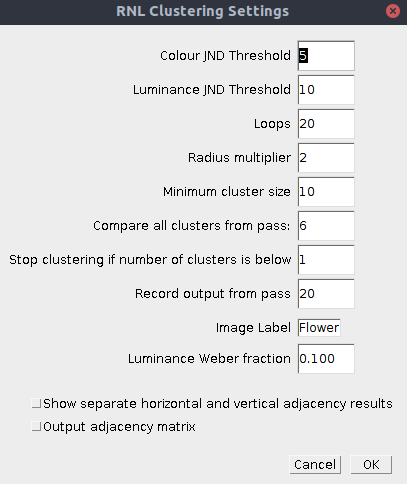
| Colour JND Threshold | The log chromatic RNL Delta-S threshold below which clusters can be combined. These numbers can be behaviourally validated, but sensible numbers are in the range of around 1-5. Set to e.g. 9999 to disable the chromatic threshold. |
| Luminance JND Threshold | The log luminance RNL Delta-S threshold below which clusters can be combined. These numbers can be behaviourally validated, but sensible numbers are in the range of around 1-10. Set to e.g. 9999 to disable the luminance threshold. |
| Loops | Maximum number of passes of the hierarchical agglomerative clustering algorithm. Images are typically clustered after around 10-12 passes, however the later passes become very fast. 20 is a suitable number for almost all images. |
| Radius Multiplier | The initial radius over which clusters are compared to their neighbours is 1 pixel. With each pass the radius can be set to get larger (simulating an increasing receptive field size). The radius is multiplied by this number with each pass, so a value of 2 means doubling the size of the receptive field with each pass. |
| Minimum Cluster Size | If a cluster is below the minimum cluster size it is forced to combine with the nearest (in chromatic and luminance Delta-S terms) cluster within the relevant radius. The minimum cluster size increases linearly with each pass so that by the final pass it is equal to the specified number. This is useful for eliminating single-pixel clusters. |
| Compare all clusters from pass | After a specified number of passes it becomes more computationally efficient to compare every cluster to every other cluster in the image (rather than searching spatially for each cluster’s nearest neighbour with ever increasing receptive field sizes). Typically this becomes optimal after approximately 5-7 passes depending on the image size. |
| Stop clustering if number of clusters is below | If the number of clusters reaches the specified value before the clustering has finished, it stops clustering at the current pass. |
| Record output from pass | This option allows the user to see the output from passes before the final pass (useful if you’re interested in seeing how the clustering progresses over subsequent passes). |
| Image Label | Specify an image label. This will be the label used in the results table, so is useful to define for subsequent statistics comparing images. |
Luminance Weber fraction | Specify the luminance Weber fraction. Unless you have behavioural data to justify a particular value, numbers in the range of 0.1 to 0.2 are typical. |
Show separate horizontal and vertical adjacency results | If ticked, the code also outputs the different horizontal and vertical pixel transition data separately (the default combines horizontal and vertical transitions) |
| Output adjacency matrix | Option for also outputting the counts of pixels of each cluster which are adjacent to each other. Useful if you wish to perform your own matrix calculations. |
Output
The RNL clustering outputs two images; first, an image with the suffix “_Cluster_IDs”, where each cluster is shown numerically from 1 to n clusters. The numbers conform to the cluster ID numbers listed in the results table. Note that is image, plus the “Cluster Results” table are required for performing the adjacency analysis on an ROI. The second image (with the suffix “_Clustered”) is a stack showing the mean cluster cone-catch values for each receptor class, and can – for example – be used for creating a false colour output image.
Two results tables are produced; “Summary Results” lists all the BSA/adjacency/average image statistics, with one line per image. “Cluster Results” lists one row for each cluster in the image, detailing average cluster statistics.
Details of the Algorithm
The algorithm uses agglomerative hierarchical clustering; at the start of clustering each pixel is its own unique cluster. Each cluster is then compared to its neighbouring clusters within a given radius (receptive field). Each cluster is then combined with its neighbour which shares the lowest Delta-S value (in chromatic/colour distance, achromatic/luminance distance, or both), only if the distances are below the respective colour and luminance thresholds. Clusters can be combined with multiple neighbours if, for example, cluster A is nearest to cluster B, but cluster B is nearest to cluster C. Meaning it is possible that a string of related colours can be combined in one pass. The algorithm then repeats the clustering over a number of passes, increasing the receptive field of the cluster comparisons with each pass. By around pass 5-7 a typical 1 megapixel image would be reduced to a few thousand clusters, at which point n-by-n cluster comparisons become more computationally efficient (conceptually similar to increasing the receptive field to the entire image).
Modifying the Algorithm
Further details of the algorithm are outlined in the original QCPA publication and suppl. material. The method for combining colour and luminance thresholds can be manually changed in the JAVA source file.
Alternative Clustering Methods
The naive Bayes clustering tool can be used for clustering in cases where you know exactly how many cluster you want/expect (and can justify this because the sample/organism clearly has a limited number of discrete colours which can easily be distinguished).