
Acuity correction is an important step in modelling receiver vision, and in the QCPA framework, controlling for the receiver’s spatial acuity, and the viewing distance. Initially developed in Matlab by Sönke Johnsen (Based on well-known Fourier math), later adapted for R and officially published as a stand-alone named ‘AcuityView’ by Eleanor Caves we have adapted AcuityView for the QCPA with some major modifications. The tool allows the user to remove the spatial frequencies (pattern information) of an image using a reverse Fourier transform, resulting in an image that only contains information above the resolution set by the visual acuity of a viewer and the viewing distance. Due to its mathematical properties AcuityView only works with rectangular images (the R version could only use square images). The user can either specify the dimension of the original image and the desired outcome in terms of MRA (Minimum resolvable angle) or, by using a size standard in the image in combination of viewer acuity and viewing distance.
This form of acuity control simply removes spatial information which would not be visible to the receiver, however it does so by creating soft, blurred images. Visual systems clearly do not see things as blurred in this way (consider people with bad eyesight who only realise how blurred their vision was after putting on prescription glasses). We therefore developed a an element in the QCPA framework which can recover sharp edges from these blurred images though use of the RNL Ranked Filter. QCPA furthermore provides the option of using a Gaussian filter for object oriented acuity modelling.
For convenience we have compiled a list of animal spatial acuities.
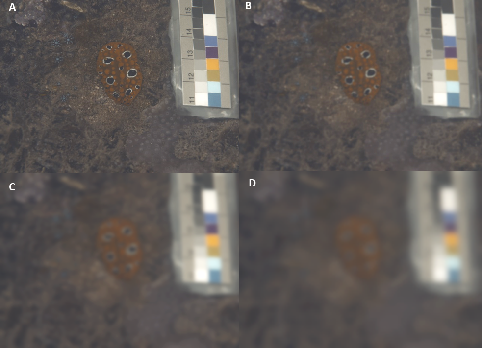
Examples of a nudibranch, modelled as seen by a triggerfish (R.aculeatus) in 5m depth at various viewing distances modelled using AcuityView. A: No acuity modelling B: 10cm C: 30cm D: 50cm (See suppl. Material for details).
Input Requirements
AcuityView works on any 32-bit stack (e.g. normalised, linear reflectance image, or cone-catch image). You must also know the spatial acuity of the visual system you’re modelling (see the tables of acuity values here), and the angular width of the image or the simulated viewing distance (in which case you also need a scale bar in the image).
Running AcuityView
Ensure the correct image is selected. You can either run this on its own (plugins > micaToolbox > QCPA > Acuity View), or as an option in the QCPA framework (plugins > micaToolbox > QCPA > Run QCPA Framework, and selecting “AcuityView” from the options).
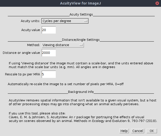
| Acuity Units | Select either “cycles per degree” or “minimum resolvable angle” depending on which is more convenient (acuity = 1/MRA) |
| Acuity Value | The number of cycles per degree, or MRA of the visual system (depending on which units you’ve selected above). See the list of animal spatial acuities. |
| Method | Viewing Distance: Acuity is calculated from a combination of the known distance to the image plane, and the width of that plane. If this is selected the image must contain a scale bar (created by drawing a line selection along a scale bar visible in an mspec image and pressing “S”). Angular Width of Image: Select if you don’t know the scale in the image, but do know the angular width of the image (this will depend on the lens/zoom factor, sensor size, and whether any image cropping has been used. In general this is less likely to be useful. |
| Distance or Angle Value | Add the respective distance or image angular width. If “viewing distance” is chosen above the units used here must match the units used in the scale bar. We recommend using millimetres for all distance measurements as default to avoid confusion. If “Angular width” is chosen above then the units here are degrees. |
| Rescale to px per MRA | This option rescales the output image to uniform number of pixels per minimum resolvable angle. This is convenient for a number of reasons, as it reduces the image dimensions without loss of spatial information. It also speeds up image processing significantly, and ensures all images not only have the same level of spatial information, but have the same effective resolution (i.e. it will make various types of pattern or image analysis more consistent). We recommend 5 px/MRA, more than this is unnecessary, any less could cause loss of spatial information. Set to zero to turn off this feature. |
Which acuity control method should I use?
If you will only ever be measuring entire (rectangular) images, and want the fastest possible processing speeds then use the AcuityView method. If you will be measuring (non-rectangular) image sections independently of their surrounding pixels, then use the Gaussian Acuity Control. If you will be comparing whole (rectangular) image sections to non-rectangular sub-sections, then also use Gaussian Acuity Control for all image processing (to keep the processing steps consistent).
Citation
If you use AcuityView for ImageJ cite the original AcuityView:
Caves, E. M., & Johnsen, S. (2018). AcuityView: An r package for portraying the effects of visual acuity on scenes observed by an animal. Methods in Ecology and Evolution, 9(3), 793–797. doi:10.1111/2041-210X.12911