
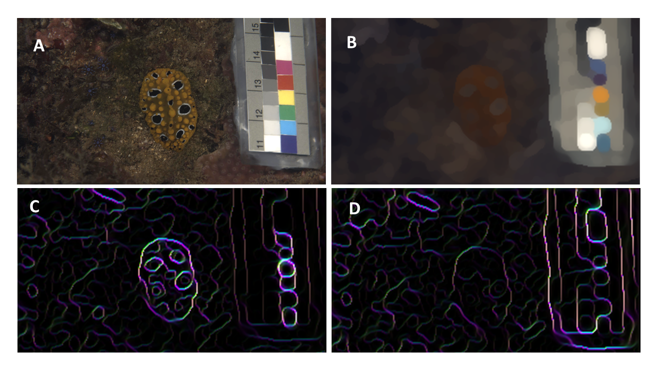
The Local Edge Intensity Analysis (LEIA) measures edge intensities across a one-pixel-neighbourhood in four directions: horizontal, vertical and both diagonals. The contrast is measured as the Euclidean distance in the log-transformed Receptor Noise Limited (RNL) colour space and provided as both chromatic and achromatic contrast between neighbouring pixels. This provides a local measure of edge contrast, which in combination with visual acuity control and the RNL ranked filter provides an approximation of centre surround field scaled edge detection. Conceptually, this is very similar to the Boundary Strength Analysis (BSA), however the major difference is that this runs on unclustered/unsegmented images (e.g. the unique case in the BSA where each pixel is its own cluster). Additionally, the output has been modified to account for the fact that in any natural image the distribution of Delta-S values will follow something like a log distribution, meaning the data should be transformed and/or measured in ways which account for this non-normal distribution.
The output images show false colour, where the hue specifies the angle of the boundary, and the intensity shows the Delta-S of the boundary.
Input Requirements
We recommend this method should be used following acuity control (FFT-based AcuityView or Gaussian acuity control) and RNL ranked filtering. This pre-processing is essential for ensuring the detected edges will be visible to the receiver at a given distance, while also recovering appropriate colour boundaries following acuity control.
The method requires a 32-bits/channel cone-catch image (di-, tri- or tetrachromatic), and the user is asked to provide the receiver-specific Weber fractions for each receptor channel (or select the species from a drop-down list if using the QCPA framework).
Zero pixel values in any of the cone channels will be ignored for the analysis. This is a useful method for measuring only sub-sections of in image. If there is any ROI currently selected only the region within the ROI will be measured.
Running the Local Edge Intensity Analysis
We recommend running this analysis as part of the QCPA framework with acuity correction and RNL Ranked Filtering applied:
Plugins > micaToolbox > QCPA > Run QCPA Framework
However, it can also be run in isolation on any cone-catch image (you will need to specify the Weber fractions yourself):
Plugins > micaToolbox > QCPA > Tools > Local Edge Intensity Analysis
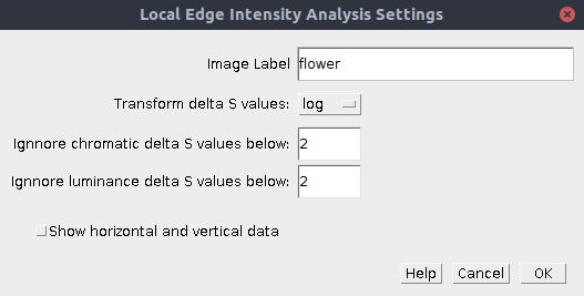
| Image Label | Select a label. This will be used in the output table. |
| Transform delta S values | none: Do not transform the Delta-S values, just use the raw output of the RNL model (note that the RNL model still uses the log-cone-catch values) sqrt: Square root transform. Sometimes the log option (below) is considered too extreme, in which case the square-root is a less aggressive choice. You can create histograms of the output images to judge the distribution yourself. log: Natural log transform the delta-S values. This tends to create a normal distribution for images of natural scenes, and is therefore probably the most sensible option. These normal distributions allow the subsequent metrics (such as coefficient of variation, skewness and kurtosis to perform better). |
| Ignore chromatic delta S values below | Sub-threshold Delta-S values are arguably imperceptible, and can therefore be eliminated. All values below this threshold are set to zero. However, this may also interfere with the distribution metrics, so is up to the user to decide whether to use this option (if in doubt, set to zero to turn this feature off). |
| Ignore luminance delta S values below | Sub-threshold Delta-S values are arguably imperceptible, and can therefore be eliminated. All values below this threshold are set to zero. However, this may also interfere with the distribution metrics, so is up to the user to decide whether to use this option (if in doubt, set to zero to turn this feature off). |
| Show horizontal and vertical dat | If ticked, output data will also be calculated for the horizontal and vertical directions independently. This could be useful when comparing patterns which are always angled in a certain direction (the images must also be standardised to show the patterns in a consistent orientation). |
Output
Two images are produced, one showing the chromatic edge Delta-S values (with the suffix “_Col_LEIA”) and another showing luminance (with the suffix “_Lum_LEIA”). Each image is a 32-bit stack of four slices, where each slice shows the values measured in different angles (horizontal, diagonal, vertical and other diagonal, labelled with symbols showing the angle: -, /, |, \). You can measure these values independently if desired. The stacks have been given false colour though lookup tables where the intensity shows the Delta-S values, and the colour varies between slice (so therefore shows angle).
A “Local Edge Intensity Analysis” results table is produced which shows measurements of Delta-S values in the image.
| Col mean | The mean chromatic RNL Delta-S values over the entire image, where at each pixel location only the maximum Delta-S across all four angles is measured. |
| Col sd | Standard deviation of chromatic Delta-S values (as above) |
| Col CoV | Chromatic Delta-S Coefficient of variation. |
| Col skew | Chromatic Delta-S skewness. Skewness is a measure of the asymmetry of the distribution of Delta-S values about the mean. Generally a higher number would imply the image has a larger proportion of high AND low Delta-S values (possibly a prediction of a salient signal). |
| Col kurtosis | Chromatic Delta-S kurtosis. Kurtosis is a measure of the degree of extreme outliers creating tails at either end of the distribution. A higher kurtosis implies very low variation in Delta-S values about the mean. |
| Lum mean | The mean luminance (achromatic) RNL Delta-S values over the entire image, where at each pixel location only the maximum Delta-S across all four angles is measured. |
| Lum sd | Standard deviation of luminance Delta-S values (as above) |
| Lum CoV | Luminance Delta-S Coefficient of variation. |
| Lum skew | Luminance Delta-S skewness. Skewness is a measure of the asymmetry of the distribution of Delta-S values about the mean. Generally a higher number would imply the image has a larger proportion of high AND low Delta-S values (possibly a prediction of a salient signal). |
| Lum kurtosis | Luminance Delta-S kurtosis. Kurtosis is a measure of the degree of extreme outliers creating tails at either end of the distribution. A higher kurtosis implies very low variation in Delta-S values about the mean. |
| Transform | Specifies which transform was applied to the Delta-S values before the above metrics are calculated (none, square-root, or natural log). |
| Col thresh | Specifies the selected chromatic Delta-S threshold, below which all values are set to zero for calculating the above metrics. |
| Lum thresh | Specifies the selected luminance Delta-S threshold, below which all values are set to zero for calculating the above metrics. |