
1. Introduction
This document describes a rigorous approach to estimating the relative spectral sensitivities of a digital camera. Our process maintains a chain of calibration, from certified calibrated light sources through to the digital camera, to ensure consistent results. Each step of the process is guided by mathematical models of the instruments, including consideration of measurement noise. We further provide a curated set of python scripts used in this workflow, available here: https://github.com/s-bear/camera-spectral-calibration. Conceptually, this procedure is much like the previously shown approach: http://www.empiricalimaging.com/knowledge-base/make-your-own-camera-callibration/. However, the approach shown here, in combination with the provided scripts, is more thorough and explains the chain of processes in much more detail. Both approaches provide almost identical results and may be more suitable to users depending on available equipment. Lastly, these approaches are not exhaustive but showcase and explain our methodology.
Briefly, spectral calibration of an instrument requires measuring a set of known spectra and inferring the instrument’s sensitivity from those measurements. For a digital camera, this means photographing a set of known spectral irradiances produced by, for example, a colour chart under a standard illuminant or a monochromator. Here we use a monochromator as our specific application requires calibration in the ultraviolet (UV) spectrum, which is not typically covered by a colour chart. The general ideas are the same in either case, and we present some results based on the X-Rite ColorChecker chart’s spectral reflectance.
Of course, maintaining a chain of calibration means we must calibrate the monochromator (or colour chart), which requires measuring its output with a calibrated optical spectrometer. The output of a monochromator is characterised by the amount of light emitted for each wavelength. In contrast, the output of a colour standard is characterised by the amount of light reflected from a given colour tile.
Note that we are aiming only for a relative spectral calibration. Specifically, we wish to know the camera’s sensitivity ratio between its colour channels within any spectral range (e.g., “the blue channel is 100 times more sensitive than red at 450-455 nm”) and between spectral ranges within any colour channel (e.g., “the red channel is 100 times more sensitive at 650-655 nm than at 450-455 nm”). Performing an absolute or photometric spectral calibration requires more sophisticated equipment and significantly more care while performing the measurements. However, the mathematical treatment would be similar to what we present here.
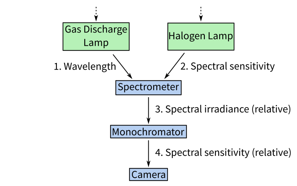
The complete chain of calibration is shown in Fig. 1. The details of the spectrometer calibration should be covered by its manual, so we treat it minimally here. The monochromator and camera calibration procedures are covered in the subsequent sections, followed by the mathematical details and some considerations on choosing suitable interpolation methods. Finally, we present the results of calibrating a Nikon D810 camera with a full-spectrum conversion.
It is essential to note that light intensity can be characterised as energy or photons. This is a crucial distinction, as photons carry different amounts of energy at a given wavelength. As a result, emission spectra or other light measurements have vastly different shapes depending on what units these are measured in. As we are only interested in a relative calibration, the calibrations can be performed in either photons or energy, as long as this is kept uniform throughout the process and across devices. However, as cameras and photometers naturally respond to energy at a given wavelength rather than photons, we recommend running the calibrations in energy, i.e., microwatts.
2. Calibrating the spectrometer
Digital optical spectrometers split incident light by wavelength across an array of photodetectors (often a linear CCD). Each photodetector element serves as a bin, counting the incident photons within a narrow wavelength band during the device’s integration time. These devices require two stages of calibration: first, a wavelength calibration to determine which spectral range each bin covers, and second, an irradiance calibration to determine the sensitivity of the photodetectors.
In brief, wavelength calibration is performed by measuring the output of a gas discharge lamp with well-known emission lines, which are used to identify which wavelengths align with which bins. After, irradiance calibration requires measuring the output of a broad-spectrum lamp with known spectral irradiance. The raw measurements are compared to the known spectrum to determine a set of calibration coefficients which map the measurement onto the true value.
In practice, these procedures tend to be included in a spectrometer’s operating software and are straightforward to execute. A spectrometer’s wavelength alignment typically changes slowly, if at all, and thus wavelength calibration only needs to be performed rarely. The device’s total spectral sensitivity depends on the spectral transmission of its light-collecting optics and the photodetector array’s sensitivity—which may depend on software settings and the ambient temperature. Best practice is to recalibrate after any change to the optical set-up (e.g. changes in optic fibre cables and auxiliary components such as cosine correctors) or any significant change to operating conditions. During fieldwork, it’s wise to regularly measure white and dark standards as a point of reference for changing conditions.
3. Calibrating the monochromator
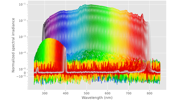
Monochromators are essentially spectrometers in reverse: a broad-spectrum light source is split by wavelength, and a system of rotating mirrors is used to focus a narrow band of wavelengths out of the device’s exit slit (typically) into an optic fibre. The calibration procedure is to couple the spectrometer to the monochromator’s output, sweep the monochromator’s nominal output wavelength along the spectral band of interest (e.g., every 5 nm from 300 to 800 nm), and record the spectral irradiance at each step. From these measurements, it is possible to compute the actual peak wavelength of each output, the total irradiance (or photon flux), and the bandwidth. They will also reveal any sidebands or broad-spectrum light leakage.
For applications that require specific irradiances or photon fluxes, these data would allow us to drive a variable neutral density filter in lockstep with the monochromator to normalise its output. Digital cameras do not require such consideration as we can simply vary the camera’s shutter speed without ill effects on the calibration procedure. Minor deviations in peak wavelength are also inconsequential here.
Monochromators require regular recalibration as their lamps’ spectral irradiance changes with age. With use, metal from the lamp’s filament will vaporise and deposit on the interior surface of the glass bulb, changing its effective spectrum. While the halogen gasses within the bulb slow the process, best practice is to recalibrate after changing the lamp or after 50 hours of use, following the guidelines for recertification of officially calibrated lamps.
4. Calibrating the camera
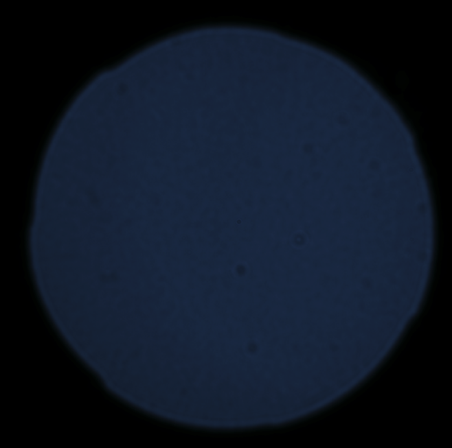
While camera designs may vary, here we assume that the camera is a typical digital camera with several broad spectral channels uniformly distributed over the image sensor area. The camera is set to photograph the monochromator output, preferably filling most of the frame. Because we are only calibrating the camera’s spectral response, it does not matter if the image is in focus—it is perfectly acceptable to put the monochromator’s output very close to the camera’s lens. It is also reasonable to calibrate a camera with no lens—though this means that any lens’s spectral transmission will need to be measured separately. The monochromator is set to each wavelength of interest in turn, and the camera is used to photograph the output. For the best signal-to-noise ratio (SNR), we want the pixels to be well-exposed but none over-exposed (Fig. 4). We target a peak at about 75% on the image histogram. The camera should be set to record RAW images in fully manual mode, including shutter speed, aperture, ISO sensitivity/gain, and white balance. While we could technically use automatic shutter speed or automatic aperture modes, in our experience, most cameras do not adjust well to a black frame with a single pure colour dot—exposure bracketing is a more reliable way to ensure at least one good exposure in this scenario.
Once all the images are recorded, we begin the data processing. Each image is converted to a standard format and cropped to show just the monochromator output. We select the highest SNR image from each exposure bracket, normalise by the exposure time, and record its mean pixel value. We analyse the entire spectral image stack to determine the fixed-pattern noise (e.g., dust or hot/dead pixels) and subtract it to determine each image’s temporal noise component (read noise and shot noise). We then use the samples along with the monochromator spectral data to infer the camera’s spectral sensitivities as a linear regression problem, described in detail below.
5. Software
Our spectral calibration software consists of several Python scripts, each for a specific step of the process, driven by settings files and all coordinated by the SCons build system for easy reproducibility. Data is stored in HDF5 files, which allow storage of multiple datasets and all relevant metadata, such as units of measure and notes about instrument settings, together in a single file. Detailed instructions are provided in the Github repository: https://github.com/s-bear/camera-spectral-calibration. Please note that these scripts are an early release (see contact details below).
The scripts are:
collate_spectra.py – which processes and collects the monochromator spectral measurements into a single file,
collate_image_stats.py – which processes and collects the statistics from a spectral image stack,
camera_resonse.py – which estimates the camera’s spectral response from the image statistics,
collate_responses.py – which collates multiple camera responses into a single Excel file for review.
Additional files are:
SConstruct – which scans the directory for settings files and schedules execution of the scripts, skipping any steps which have already been completed,
environment.yml – which includes the list of software dependencies required to run the scripts.
6. Mathematical Models
6.1 Spectrometer Measurements
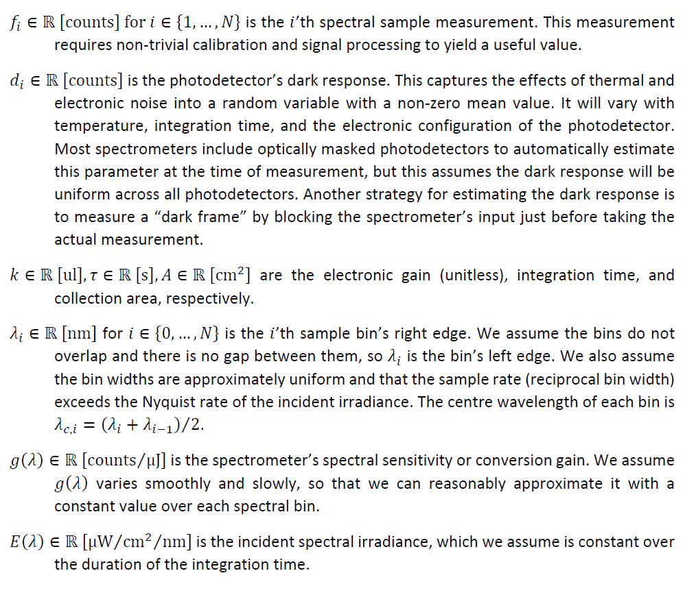
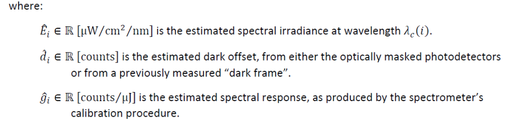
A typical digital optical spectrometer’s response may be modelled by:
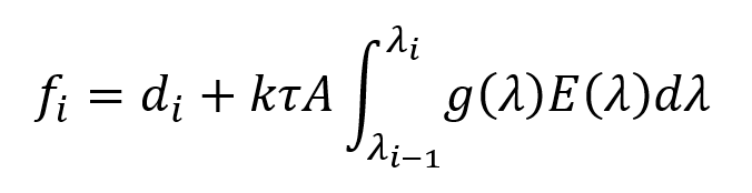
where:
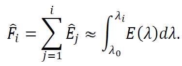
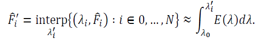
6.1.1 Resampling spectral measurements
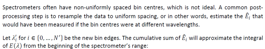


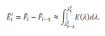
The accuracy of this method depends on how well the interpolation function can estimate the original underlying spectral irradiance. If the original sampling rate (reciprocal bin width) exceeds the Nyquist rate of the irradiance, then an appropriate interpolation filter will result in minimal resampling error.
6.2 Camera calibration
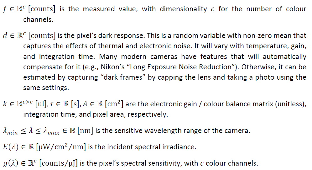
The spectral response of a typical digital camera’s pixel may be modelled as:
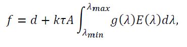
where:
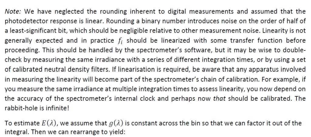
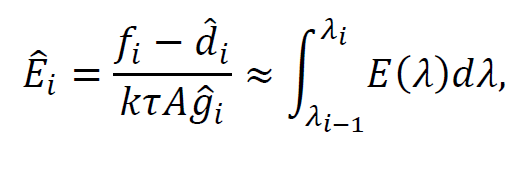
Note: We have assumed the pixel response is linear. This is not true in general and is explicitly untrue with most common image and video formats. In practice, it is necessary to use the camera’s raw image format and develop them into 16-bit TIFFs with a linear profile. Such images will not “look good” because the human visual system is non-linear, but they will allow error-free mathematical manipulation!
Unlike the spectrometer case, here we wish to determine 𝑔𝑔(𝜆𝜆) and there is no easy way to extract it from the integral. It is possible to “un-mix” an integral of the product of two functions using deconvolution techniques, but only in very specific scenarios. Here, however, we benefit from moving into the discrete (sampled) domain as these models translate into linear systems of equations. Of course, it would be impossible to solve for the spectral irradiance from a single measurement, so we measure many known spectral irradiances that span the spectral sensitivity range of the camera.

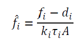

where:
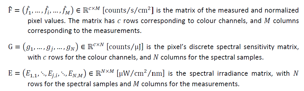
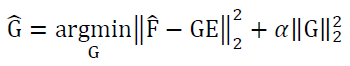
In practice, we use a monochromator to generate spectral irradiances with smooth, narrow bands that we can sweep over the sensitive range of the camera. The bandwidth of our monochromator is approximately 10 nm full width at half-maximum (FWHM), so we step its output by 5 nm for each measurement. This is significantly less than our spectrometer’s resolution of ~ 1 nm, leading to an under-determined system when we try to solve Eq. 9 for G. That is, there are infinitely many solutions that we could plug-in for G that would satisfy the system. By assuming that the spectral response is smooth and zero outside the measured region, we can apply ridge regression to select the “minimum energy” solution from that set.
For all queries regarding these scripts, don’t hesitate to get in touch with Samuel B. Powell: samuel.powell@uq.edu.au
Text written by Samuel B. Powell (lead) & Cedric P. van den Berg
Python scripts written by Samuel B. Powell